Trading Research & Development
We selected four studies for this site. They cover the cost of a SUI short liquidation, where to enter on an ETH pullback, how to select strategy parameters and why simulated annealing can lead to overfitting.
We lost $1,000 in 8 seconds
Initial margin $1,000
The exchange made $750 on this liquidation — three quarters of our initial margin. We literally gifted it that money.
Why does that matter? We entered at 4.2358. The highest traded price during the second of liquidation was 4.2410. Even closing at that high would account for about $250 of loss from the price move. The remaining $750 is the difference between the margin we lost and that market-price comparison.
In a liquidation, settling with the trader and subsequently closing the position in the market are separate operations. If the exchange closes the position at a better price than its takeover price, it keeps the difference. In our case, that $750 went to the exchange’s bottom line: our loss became its earnings.
SUI second by second
- Short entry
- 4.2358Our fill matched the low of this second.
- Trades during the liquidation second
- 4.2401–4.2410Even the highest trade was only 0.123% above our entry.
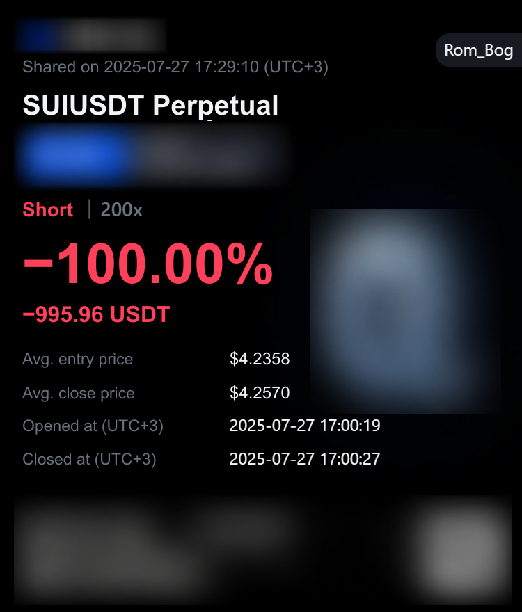
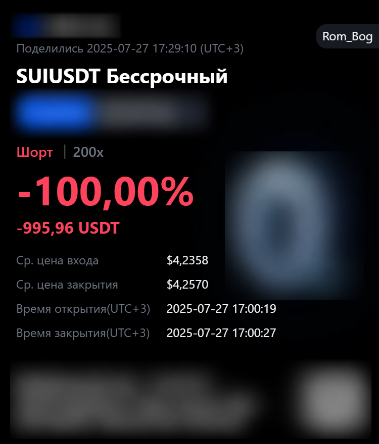
The receipt shows an average closing price of 4.2570 USDT. This is the price that exhausts the initial margin. At 200× leverage, the margin is 0.5% of the position value. A rise of that size from our short entry uses up the entire margin before fees.
In our case, the exchange bought back the short during the second marked candle, at 17:00:27 UTC+3. The buyback fell within that second’s traded range of 4.2401 to 4.2410 USDT.
If not always, then in most cases, liquidation is the most costly way to exit a position. Exit earlier to preserve the remaining margin.
Parameter selection
Look for a region of strong results, rather than a single record.
Two settings vary in this teaching example:
- AMoving average period: 10–74 bars.
- BPosition holding period: 1–41 bars.
One-bar steps give pairs. Each pair is scored on the same history under the same conditions. Height and colour show the score.
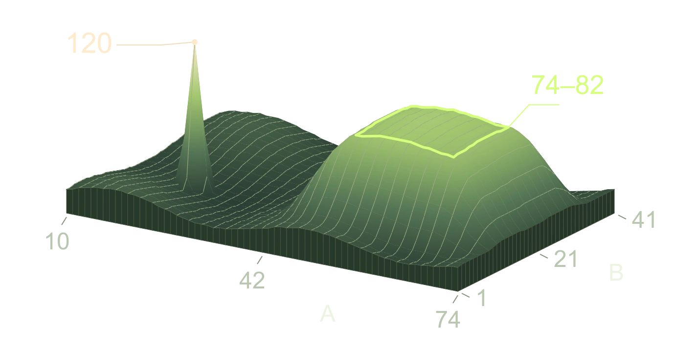
Isolated peak
The highest point scores 120. Change either parameter by one step and the score falls to 70. That record is too sensitive to an exact setting to select it solely because it ranks first.
Region for further search
Nearby, another region contains 255 neighbouring combinations scoring between 74 and 82. Strong results persist across many similar settings. This makes the region a candidate for testing on a different period.
Keep the settings fixed and rerun the same grid on a period held out of the search. Compare the two plots. Does the same group of neighbouring settings still score well?
A record tells you which pair won once. A plateau that reappears on fresh data gives you a reason to trust a range of settings.
Our level for a pullback
Using our own backtesters and more than ten years of market data, we calculated a proprietary level and identified the zone where, provided the current trend continues, the ongoing correction is most likely to end — reaching its greatest pullback depth before movement in the trend direction resumes.
We place limit orders at the boundary of this zone. Below are ETH examples.
The simulated annealing algorithm
A record on one dataset. Failure on another.
For competitive programming enthusiasts. If the objective is to extract the highest score from a given dataset, a strong search algorithm can produce a convincing result. A trading model also needs to work on data the search has never seen.
Why accept a worse score?
In this synthetic experiment the search starts with a set of weights θ. Change one weight at random and score the new set θ′ on the same synthetic sample A. The score S is the percentage of correct forecasts. An improvement always goes through. Allowing the occasional loss lets the search cross a valley between two peaks.
The name comes from the controlled cooling of heated metal. In the search, temperature T sets the scale for an acceptable drop in score. As T falls, the same drop becomes harder to accept. The current weights can move downhill while the best weights found so far stay on record.
The experiment starts with twelve zero weights. We choose one of them with equal probability and add a uniform draw between −0.8 and +0.8. If the result falls outside the range from −4 to +4, we use the nearest endpoint. Across 6,000 proposals the temperature falls from 18 to 0.09 percentage points.
Change in score
Probability of accepting the move
Cooling schedule, with the first proposal at step zero
In one recorded step, the hit rate fell by 11.11 percentage points. At a temperature of 17.98, the probability of accepting that loss was 53.9%. The random draw of 0.47 fell below the threshold. The current score dropped to 50%, while the best stayed at 61.11%.
A trading rule in a random market
Suppose we observe twelve weighted criteria before each trade. We add their weighted values and go long if the sum is zero or positive, or short if it is negative. After entry, price moves ten basis points up or down with equal probability, independently of all twelve criteria.
Close each trade after one bar. One basis point is 0.01% of the position. Entry and exit together cost two basis points. A correct call earns eight basis points net and a wrong call loses twelve. Write J for the net result per trade and h for the probability of a correct call.
Expected net result in basis points
Hit rate needed to break even
Each new move in this experiment is independent of the criteria. Once the weights are fixed, the probability of a correct call is one half.
Expected net result on a new trade, in basis points
What survives the next trade?
On sample A, the search tries 6,000 changes to the weights against the same 18 trades, keeping the set with the highest hit rate. We freeze those weights and apply them to the next 1,800 synthetic trades in B. Both samples use the same price process and trading costs.
18 of 18 directions correct
911 of 1,800 directions correct
How precisely does B estimate the hit probability? Let n be the number of test trades and h the probability of a correct call. For independent trades with a common h, the two-sided 95% Wilson interval consists of the values of h satisfying the inequality below.
Observed hit rate on B
95% Wilson interval
The interval includes 50%. Even its upper limit is below the 60% needed to break even. Applying the payoff per trade to the two endpoints gives a 95% interval of -2.34 to -1.42 basis points for the expected net result.
Wilson interval derivation · NISTOverfitting
Fix a rule before seeing the outcomes. With independent, equally likely up and down moves, its chance of calling all 18 trades correctly is 1 in 262,144. When we choose the weights after seeing the outcomes, how many different sequences can we fit perfectly?
Each of the 18 trades is a point in 12 dimensions, one coordinate per criterion. A vector of weights defines a hyperplane through the origin. The sign of the weighted sum places each point on the long or the short side. Cover’s theorem counts the assignments for which a hyperplane puts every point strictly on its assigned side.
The theorem requires every set of 12 feature vectors to be linearly independent. We checked all 18,564 such sets in A. Scaling the weights by a sufficiently small positive factor brings them within the search bounds while preserving every forecast.
Perfectly separable sequences on A
Chance of a perfect fit on A
What does the search actually find? On 32 new training samples, with 6,000 proposals per sample, it gets at least 17 of 18 calls right in 24 runs and all 18 right in 9. The search has a finite budget. After selection, each fixed rule still has a 50% chance of calling the next move correctly.
Cover’s counting theorem · Theorem 1Why roughly three blocks in four lose money
Split B into 100 consecutive blocks of 18 trades. The fitted rule loses money in 77 of them. For this fair-coin model we can also calculate that risk exactly.
For independent price moves, the number K of correct calls in 18 trades follows a binomial distribution with success probability one half. Ten wins still leave a loss. Eleven are enough for a profit. Each binomial coefficient counts the ways to place k correct calls among the 18 trades.
Probability of a losing block
This probability belongs to the synthetic market defined above. For a live rule the hit rate, payoff and costs have to be estimated on market data set aside before tuning. Changing the rule after seeing that result makes the period part of the search.
The search solved the task it was given: finding settings for A. Alongside useful relationships, it may have fitted the accidental features of those data. That is overfitting. A stronger search and a more persistent pursuit of a record can make it easier to mistake that fit for a robust result.